03. Lesson Map and Fusion Flow
Lesson Map
Overview of the Kalman Filter Algorithm Map
For your reference: a map of the Kalman Filter algorithm! Keep an eye out, because we'll add a little bit more detail to this later.
Imagine you are in a car equipped with sensors on the outside. The car sensors can detect objects moving around: for example, the sensors might detect a pedestrian, as described in the video, or even a bicycle. For variety, let's step through the Kalman Filter algorithm using the bicycle example.
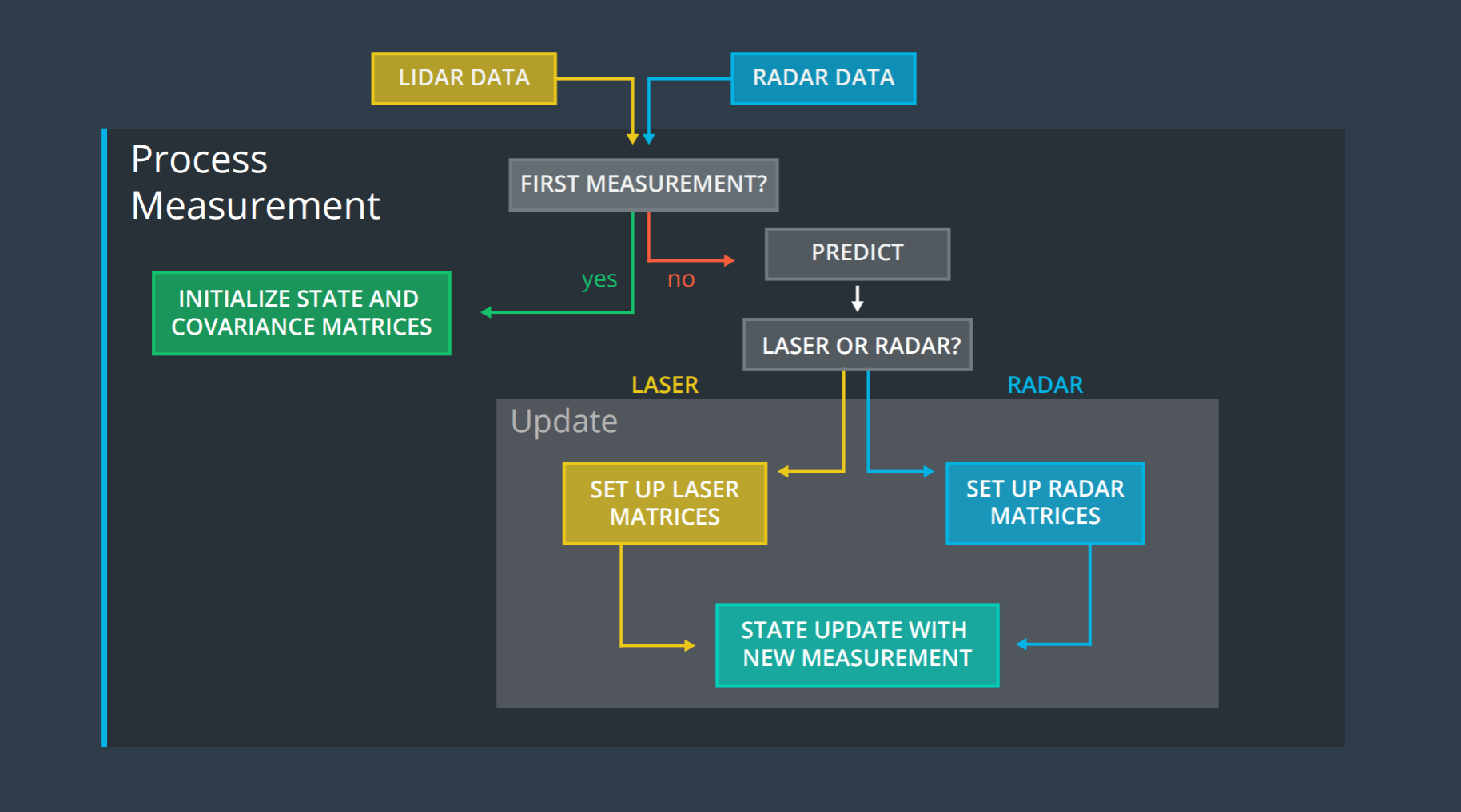
The Kalman Filter algorithm will go through the following steps:
- first measurement - the filter will receive initial measurements of the bicycle's position relative to the car. These measurements will come from a radar or lidar sensor.
- initialize state and covariance matrices - the filter will initialize the bicycle's position based on the first measurement.
- then the car will receive another sensor measurement after a time period \Delta{t} .
- predict - the algorithm will predict where the bicycle will be after time \Delta{t} . One basic way to predict the bicycle location after \Delta{t} is to assume the bicycle's velocity is constant; thus the bicycle will have moved velocity * \Delta{t} . In the extended Kalman filter lesson, we will assume the velocity is constant.
- update - the filter compares the "predicted" location with what the sensor measurement says. The predicted location and the measured location are combined to give an updated location. The Kalman filter will put more weight on either the predicted location or the measured location depending on the uncertainty of each value.
- then the car will receive another sensor measurement after a time period \Delta{t} . The algorithm then does another predict and update step.